From Trial Records and Protocol Text to an Explainable Site Recommender on the Arango Contextual Data Platform

Provisioning the Arango Contextual Data Platform and Picking Your Clinical-Trial Data

Prerequisites

Three things must be in place before any code runs:

1. Access to the platform with the Agentic AI Suite enabled (AutoGraph and Ada are enterprise-tier, requested through the demo page)
2. Python 3.11+
3. An OpenAI API key

Install the dependencies from requirements.txt, then copy .env.example to .env and fill in your values:

# Arango Contextual Data Platform
ARANGO_HOST=https://your-deployment.arango.ai
ARANGO_DB=your_database_name
ARANGO_USER=your_username
ARANGO_PASSWORD=your_password

# Provider for LLM and embeddings
OPENAI_API_KEY=your_openai_key

# AutoGraph Retriever (dosage variable)
# Find the service ID in the AutoGraph interface under your deployed Retriever service.
RETRIEVER_HOST=https://your-deployment.arango.ai
RETRIEVER_SERVICE_ID=arangodb-graphrag-retriever-xxxxx

Confirm the connection before any data lands:

from arango import ArangoClient
import os

client = ArangoClient(hosts=os.environ["ARANGO_HOST"])
db = client.db(
    os.environ["ARANGO_DB"],
    username=os.environ["ARANGO_USER"],
    password=os.environ["ARANGO_PASSWORD"],
)

Choosing Your Dataset

The recommender needs two things from a data source: structured records to build the study, site, and investigator nodes, and high-quality free-text fields for semantic search. Any source that provides both can support the pipeline, so the quality and relevance of the text matter more than the size of the dataset.

This build uses AACT by default, the public database behind ClinicalTrials.gov and maintained by the Clinical Trials Transformation Initiative. It is a strong fit because both structured and text data are available in a single download. The tables provide the graph structure, while fields such as protocol summaries and eligibility criteria provide the text used for embeddings. The build reads the required tables from aact_sample/.

Because AACT covers the full registry, the pipeline uses a focused therapeutic-area slice to keep the build practical on a laptop. The default slice contains breast cancer trials with ACTIVE_NOT_RECRUITING or RECRUITING status, covering roughly 1,688 studies and 23,000 facilities. This filter is configurable through ACTIVE_STATUSES in src/ingest.py, and the ClinicalTrials.gov API v2 can return the same slice without requiring a local AACT copy.

The Synthetic Performance Layer

AACT records which sites participated in a trial, but not how well they performed. To fill that gap, the pipeline generates performance metrics for each site, including enrollment rate, activation time, success score, and trial count, using random.seed(42) for reproducibility. In a production system, these values would come from a CRM or clinical trial management system. This is one of two synthetic data layers in the pipeline, and because it directly affects ranking, it is highlighted here and revisited in the limitations section.

Modeling and Merging the Data Shapes with Arango AutoGraph

src/ingest.py builds the database in three steps; the structured graph, the embeddings, and the performance layer, defining the schema first so a rerun creates no duplicates.

Defining the Schema

The schema holds four document collections, studies, facilities, investigators, and conditions, plus one edge collection joining studies to sites and sites to investigators.

graph = db.create_graph("site_topology")
graph.create_edge_definition(
    edge_collection="site_relationships",
    from_vertex_collections=["facilities", "investigators", "studies"],
    to_vertex_collections=["facilities", "investigators", "studies", "conditions"],
)

A named graph, site_topology, sits over the edges and makes them traversable with AQL.

The four document collections hold the nodes and the single edge collection holds every relationship, which keeps the graph definition small enough to reason about at a glance.

Embedding Configuration

The pipeline uses the same embedding model, text-embedding-3-small (1,536-dimensional cosine vectors), for both ingestion and querying. Using different models would make similarity comparisons unreliable. Each embedding combines the study title, summary, eligibility criteria, and detailed description, giving the search the richest protocol context available in AACT.

doc["embed_text"] = f"{doc['brief_title']} {doc['summary']} {doc['eligibility_criteria']} {doc['detailed_description']}"

The vector index builds over that field with a cosine metric after every embedding is stored, so it trains on the complete set.

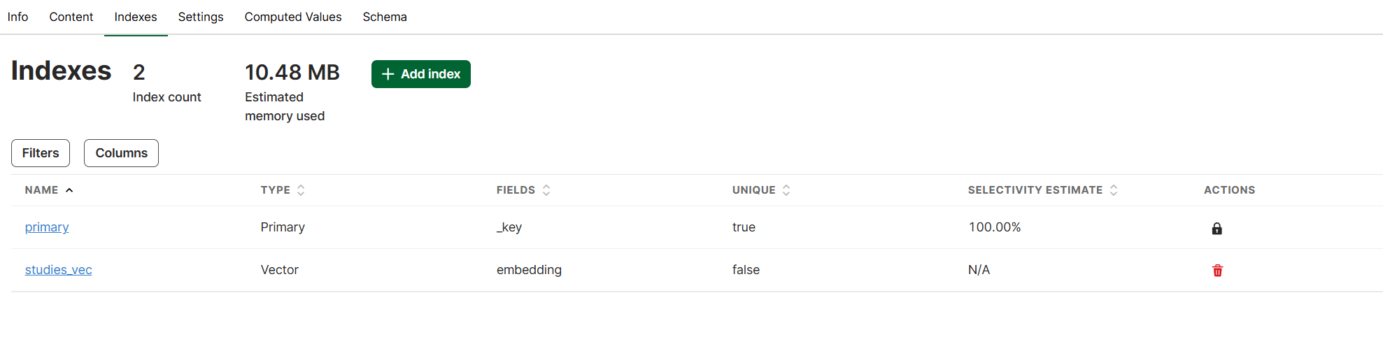
With the index in place, a new protocol can be compared against all 1,688 stored studies in a single similarity call, which is the first stage of the recommender.

Ingesting the Graph

The structured data is loaded in stages: studies with their embed_text, facilities with performance metrics, investigators, and finally the relationships. Studies are linked to facilities by nct_id, and facilities to investigators by facility_id, turning shared IDs into directed edges in site_relationships.

This is the shape the recommender walks at query time: start from a study, step outward along the edges, and land on the facilities that ran it.

Adding Population Context by Geography

Two of the five variables, prevalence and demographics, are absent from AACT. They come from federal data keyed by county, not by trial, so they cannot ride the same ingest. src/enrich.py runs a second pass that joins them onto the site nodes through geography: for each US facility it reads the latitude and longitude already loaded from AACT, resolves the county through a geocoding lookup, and attaches that county’s cancer prevalence from CDC PLACES alongside a median-age signal.

county_fips = latlon_to_fips(fac["latitude"], fac["longitude"])
db.collection("facilities").update({
    "_key": fac["_key"],
    "county_fips": county_fips,
    "cancer_prevalence": prevalence.get(county_fips),  # real, CDC PLACES
    "median_age": synthetic_median_age(county_fips),   # generated
})

A site stops being a bare location and gains a catchment, the population a feasibility team actually recruits from.

Ingesting Protocol Documents via AutoGraph

Protocol text follows a separate ingestion path. AutoGraph works with unstructured documents, so src/export_docs.py first converts each study’s structured fields, summary, eligibility criteria, and intervention text into plain text documents. That folder is then uploaded to a new AutoGraph project to start the pipeline. For a corpus of this size, the default import settings are sufficient.

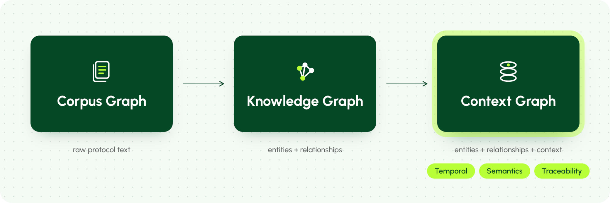
AutoGraph then analyzes the documents and determines the best way to process them. It samples the corpus, identifies the knowledge domains it contains, and evaluates their complexity. In this case, the breast cancer protocols form a rich, focused dataset, so AutoGraph groups them into a single cluster and builds a full graph of entities and relationships rather than using a simpler vector-only approach.

Once the build completes, the Context Graph dashboard shows what was created. The corpus graph holds the 50 protocol documents in a single cluster, and the knowledge graph extracted from them contains 2,412 entities and 6,187 relationships. This gives you a clear view of the structure that now backs every query.

The result is a context graph built in three stages. A corpus graph captures the documents, a knowledge graph extracts the entities and the relationships between them, and a context graph layers on semantics, time, and traceability. Unlike a plain structured graph, it links clinical concepts across protocols, which is what lets the recommender explain why a site fits rather than just ranking it.

The Retriever shows the payoff. Ask it for dosage across the similar trials and it returns specific, cited values from the source material rather than an ungrounded summary, pulled from intervention text that the structured tables do not capture. The resolver runs this in Deep Search mode, which performs a multi-step search across the entire knowledge graph rather than a single neighborhood.

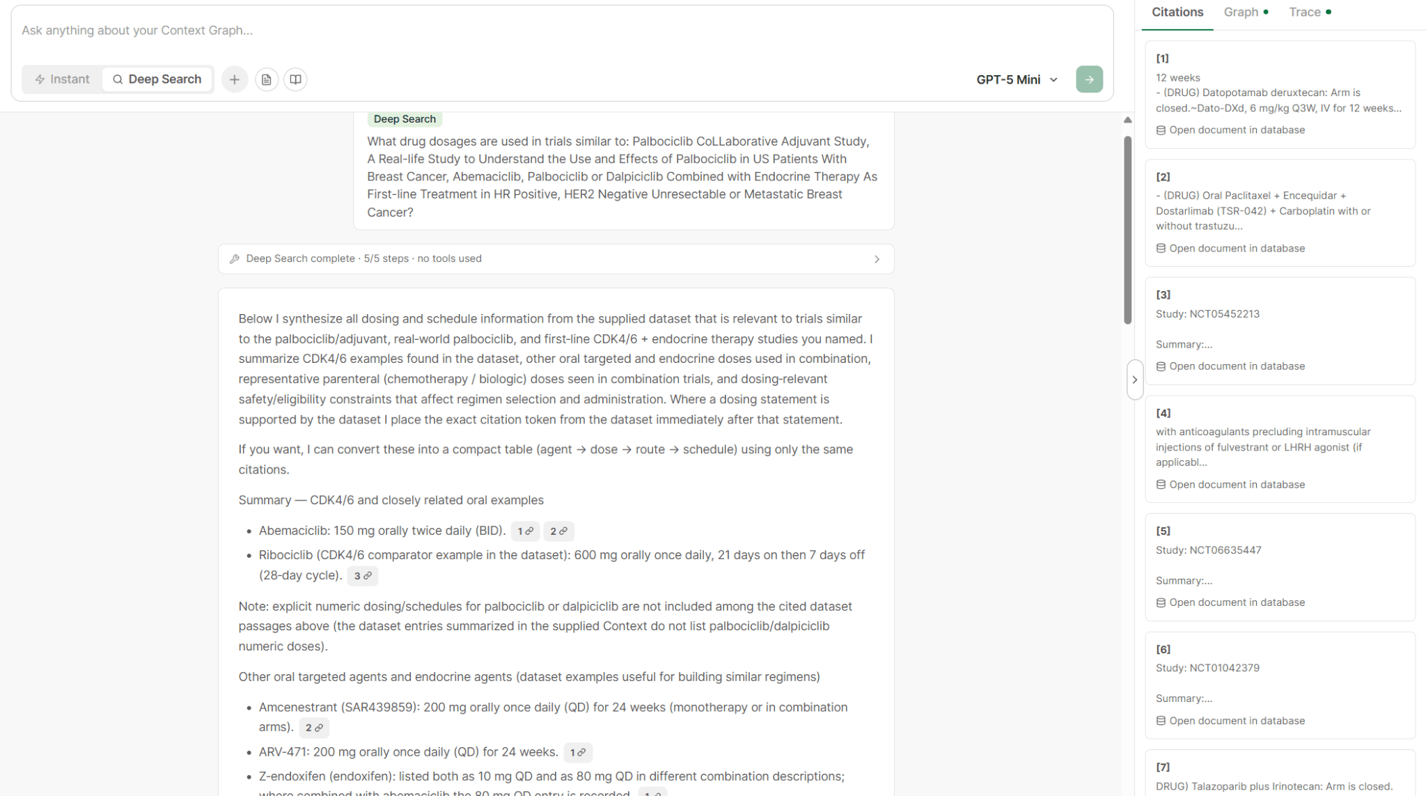
This goes beyond retrieving text. During ingestion, AutoGraph extracts structured information from each protocol against the domain ontology, identifying drugs, dosages, and their relationships and storing them as nodes and edges in a context graph. A detail like ribociclib at 600 mg once daily, 21 days on and 7 days off becomes a queryable fact linked to its source trial and backed by a citation. If the corpus contains no dosage, the Retriever says so rather than filling the gap, keeping the result grounded and giving GraphRAG a clear advantage over plain vector search.

The resolver then uses this context graph alongside the structured database, so dosage contributes directly to the recommendation alongside the four variables returned by the AQL query.

Recommending a Site Across Documents, Graph, and Vectors

The data layer is ready. Studies carry embeddings, facilities connect through the graph and hold performance and population data, and AutoGraph models the protocol text. A new protocol arrives, and src/resolver.py answers which sites fit best, and why.

The Marquee AQL Query

The query runs in two stages so the vector search keeps its own top-level SORT and LIMIT, which APPROX_NEAR_COSINE requires, with the traversal and scoring after it. The weights and the neutral defaults are passed in as bind parameters; their working values are listed in the comment at the top.

// Weights: protocol 0.35, site success 0.30, prevalence 0.20, age 0.15
// Neutral defaults for sites without geo data: prevalence 0.3, age 0.5
LET similar = (
  FOR s IN studies
    LET sim = APPROX_NEAR_COSINE(s.embedding, @vec)
    SORT sim DESC
    LIMIT 5
    RETURN { nct_id: s.nct_id, title: s.brief_title, similarity: sim }
)
LET sites = (
  FOR study IN similar
    FOR v IN 1..1 OUTBOUND CONCAT("studies/", study.nct_id) GRAPH "site_topology"
      FILTER IS_SAME_COLLECTION("facilities", v)
      FILTER v.success_score != null
      LET has_geo = v.cancer_prevalence != null
      LET prevalence_score = has_geo ? (v.cancer_prevalence / 15) : @neutral_prev
      LET age_score = (has_geo AND v.median_age != null)
        ? ((50 - ABS(v.median_age - 40)) / 50) : @neutral_age
      LET composite = (study.similarity * @w_protocol)
        + (v.success_score * @w_perf)
        + (prevalence_score * @w_prev)
        + (age_score * @w_age)
      COLLECT
        name = v.name, city = v.city, country = v.country,
        success_score = v.success_score, prevalence = v.cancer_prevalence,
        median_age = v.median_age, has_geo_data = has_geo
      AGGREGATE score = MAX(composite),
        via_similarity = MAX(study.similarity),
        prev_sub = MAX(prevalence_score),
        age_sub = MAX(age_score)
      SORT score DESC
      LIMIT 10
      RETURN {
        name, city, country, success_score, prevalence, median_age, has_geo_data,
        composite_score: score, matched_similarity: via_similarity,
        prevalence_score: prev_sub, age_score: age_sub
      }
)
RETURN { similar_studies: similar, recommended_sites: sites }

APPROX_NEAR_COSINE compares the incoming protocol against every stored one and returns the five closest matches. The @vec bind parameter is that protocol’s embedding, which resolver.py generates before the query runs. The graph then takes a single hop from each matched study to the facilities that ran it, since the site_topology edges point from studies to facilities. CONCAT("studies/", study.nct_id) builds each document handle inline, which works because a study’s key is its NCT ID.

Sites are ranked on a weighted score across protocol similarity, site performance, population data, and trial history, and the query returns each sub-score so the ranking can be broken down rather than taken on faith. Where population data is missing, neutral defaults keep a promising site in the running at lower confidence; the median_age guard ensures a site with geo data but no age value falls back to that neutral value instead of scoring zero.

The same query runs from src/resolver.py, which embeds the incoming protocol, passes the vector in as the @vec bind parameter, and formats the ranked result.

Firing a Placement

Run the resolver against the sample protocol, a Phase III study of palbociclib plus endocrine therapy in HR-positive, HER2-negative breast cancer:

python src/resolver.py data/protocol_sample.json

It returns four parts: the ranked sites, the evidence behind them, the reasoning, and a confidence signal.

=== RECOMMENDED SITES ===
Weights: protocol 35% · success 30% · prevalence 20% · age 15%

1. Avera Cancer Institute-Aberdeen -- Aberdeen, US     overall 0.847
   protocol 0.826 · success 0.97 · prevalence 0.62 · age 0.956
2. Marin Cancer Center -- Greenbrae, US                overall 0.845
   protocol 0.826 · success 0.91 · prevalence 0.70 · age 0.95
3. CAMC Cancer Center -- Charleston, US                overall 0.844
   protocol 0.826 · success 0.92 · prevalence 0.66 · age 0.982

=== EVIDENCE PASSAGES ===
- PALbociclib CoLlaborative Adjuvant Study (0.826)
- A Real-life Study ... Palbociclib in US Patients With Breast Cancer (0.81)
- Abemaciclib, Palbociclib or Dalpiciclib ... HR+/HER2- Metastatic Breast Cancer (0.809)

=== DOSAGE EVIDENCE (AutoGraph context graph) ===
- Abemaciclib: 150 mg BID, orally, 20-24 weeks (with Z-endoxifen or ARV-471)
- Ribociclib: 600 mg once daily, 21 on / 7 off (28-day cycle)
- Capivasertib: 400 mg twice daily, 4 on / 3 off
(3 distinct dosage statements)

=== REASONING ===
Avera leads on site success (0.97), outweighing Marin's stronger prevalence.
CAMC's age match isn't enough to close its gap. All sites carry geo data.

=== CONFIDENCE ===
high -- strong match, sufficient sites, complete data

=== RETRIEVAL STATS ===
top similarity : 0.826 · vector hits : 5 · depth : 1 · sites : 10 · time : 22.0s

The confidence score reflects the quality of the recommendation. It drops when protocol matches are weak, too few similar studies are found, population data is missing, or dosage context is unavailable. When confidence is low, the system makes that clear instead of overstating the result.

Why the Semantic Match Matters

The strongest evidence comes from the top matching protocol. Although the sample mentions only palbociclib, its closest match, with a score of 0.809, is a trial involving three CDK4/6 inhibitors with endocrine therapy in the same patient population. The match is driven by shared clinical meaning, including drug class, patient population, and treatment approach, rather than exact keyword overlap.

A graph database such as Neo4j can connect studies to sites and traverse those relationships well. What it cannot do on its own is judge how closely a new protocol matches past trials in meaning and fold that judgment into the same traversal. This is where Arango AutoGraph adds value. Vector search and graph traversal run together in the same query engine, allowing the system to combine semantic similarity with each site’s connections to relevant trial history. There is no separate vector store to manage or keep in sync. The complete ten-site recommendation is available in data/recommendation_output.json.

Ask Ada in Plain English

Ada, Arango’s AI Digital Assistant, can query the same data without writing AQL. For example, ask:

“Which facilities in the United States have a cancer prevalence above 8 and a median age over 40? Show name, city, prevalence, and age.”

Ada plans the query, runs it against the same enriched data the Python resolver uses, and returns the results in plain language, here as a table of matching US facilities.

The same contextual layer serves both a Python resolver and a natural-language question from a program lead who has never written AQL. One store, two front doors.